Causal graphs (often called DAGs) are used a lot in epidemiology. Until now, my approach to drawing them has been limited to pen and paper or taking a screenshot of Dagitty (another option I decided against pretty quickly was spending hours trying to do it in Word). Since I’m in the habit of using RMarkdown for any writing that needs figures/tables/stats, and recently had to write some coursework with a lot of causal graphs, I’ve had a chance to figure out a nice way to make them in R.

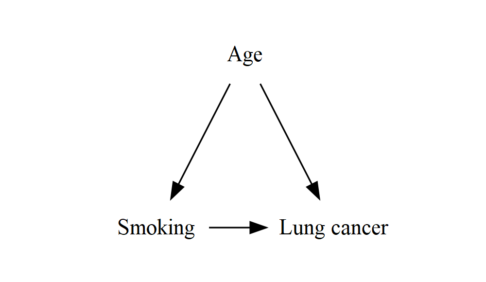
This is exactly what I wanted – just text, boxes and arrows, like you’d see in a classy book. In this post I’ll walk you through how this was done. In short, DiagrammeR lets you specify the structure of a DAG (what the nodes are and how they’re connected) with a fairly readable and understandable markup language, and it works out the layout mostly automatically. With a few tricks, it’s turned out to be surprisingly capable of handling a lot of common causal structures and drawing them in a way that will make sense to an epidemiologist.

If you just want a good starting point for quickly whipping up a decent DAG of your own, you can skip ahead to the finished example and summary at the end, but if that’s a bit overwhelming I’ll walk you through how I got there, step by step. I’m going to assume you’re already familiar with both R and causal graphs.

DiagrammeR

We’re going to use the DiagrammeR package, which is made for drawing graphs in general, not specifically causal graphs. If you want to do more complex things like analyse the properties of DAGs and the statistical and causal relationships that they imply, you might want to look at more specialised packages like dagitty and ggdag. However, these tools can be overkill if all you need is to create a visual diagram – hence this post!

All you need to follow along is the DiagrammeR package:

install.packages("DiagrammeR")

Under the hood, DiagrammeR uses Graphviz (or at least, that’s what we’re going to use here), a tool that’s been around for nearly 30 years for describing and drawing graphs using code. You don’t need to know a lot of it to get started, so I’m only going to touch on the bare minimum here. If you want to learn more, the DiagrammeR documentation explains things pretty well. But this is definitely not a prerequisite for following this post.

Starting out

Let’s start with a tiny directed graph, with just two nodes and an arrow between them.

DiagrammeR::grViz("
digraph {
  graph []
  node []
    A
    Y
  edge []
    A->Y
}
")

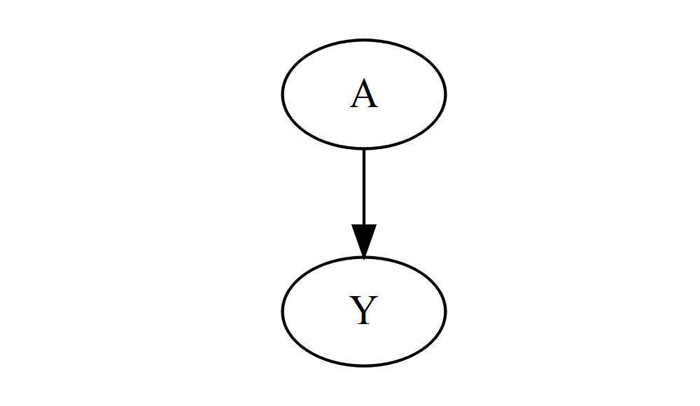
This doesn’t look very impressive yet, but it shows you the basic building blocks: to draw a graph, we call the DiagrammeR::grViz function, and pass in a single string of text that defines the entire graph. This might look a bit intimidating, but you can ignore most of it for now – just notice the list of nodes and the list of edges. Here, there are two nodes (A and Y), and one edge (A->Y) that connects them. This is all you need to represent the most complex DAG you can think of – everything else is just cosmetic. Play around with adding some nodes and edges, if you like. (If the layout starts looking wonky as you add more stuff, don’t worry – we’ll address this later!)

OK, but how do I make this actually look good?

Step by step, we’ll tweak this until it looks like the graph at the top of the post – so I’m going to assume that’s what you want yours to look like. If not, you’ll probably still learn something from this post, but it might take a bit more tweaking to get what you want.

For a start, let’s remove those circles. This is a small first step, but it’ll introduce you to an important bit of new syntax:

DiagrammeR::grViz("
digraph {
  graph []
  node [shape = plaintext]
    A
    Y
  edge []
    A->Y
}
")

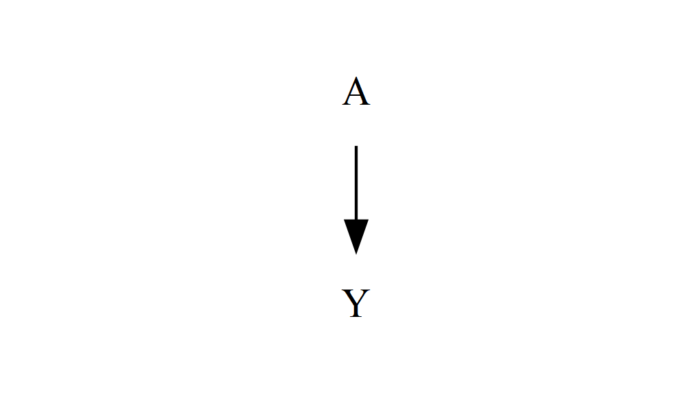
All we’ve done is set an attribute inside the square brackets after node that were previously empty: shape sets the shape of the enclosure around each node (the default is oval) – plaintext means no enclosure, just text. There are lots of possible shapes – you can see some of them in the DiagrammeR documentation, and even more in the more in-depth Graphviz documentation. We only need two: plaintext and box.

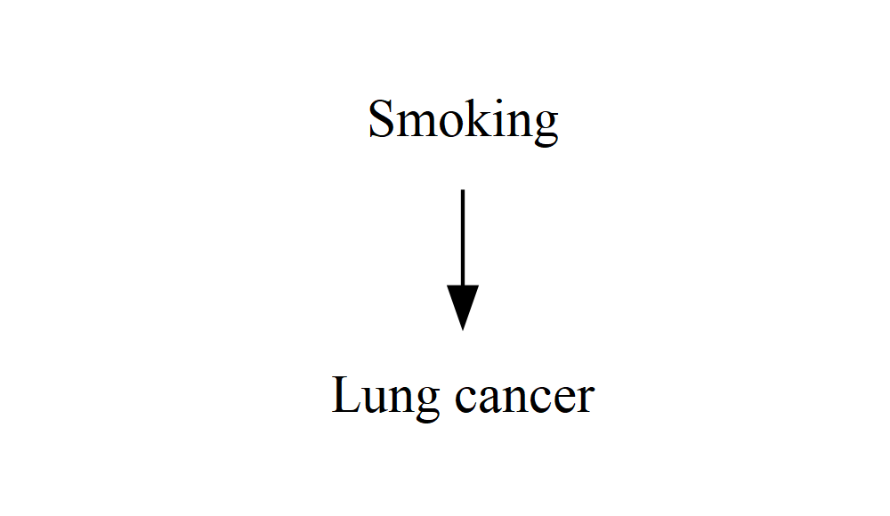
Adding longer names

If we want each node to say something longer and more descriptive than “A” and “Y”, we can add a “label” to each node – internally, they’re still called A and Y, so the edge definitions can stay the same, but they’ll appear as “Smoking” and “Lung cancer”. We could also change “A” to “Smoking” everywhere, but doing it this way means that if we want to change how something is worded, we only need to change it in one place (instead of in every single edge definition).

DiagrammeR::grViz("
digraph {
  graph []
  node [shape = plaintext]
    A [label = 'Smoking']
    Y [label = 'Lung cancer']
  edge []
    A->Y
}
")

Bigger diagrams and layout

Now, chances are you want to draw causal diagrams with more than two things, and that means you’re going to need to care about layout. You might have already discovered this if you took some time to play around earlier, but the default layout doesn’t always make a lot of sense:

DiagrammeR::grViz("
digraph {
  graph []
  node [shape = plaintext]
    A [label = 'Smoking']
    Y [label = 'Lung cancer']
    C [label = 'Age']
  edge []
    A->Y
    C->A
    C->Y
}
")

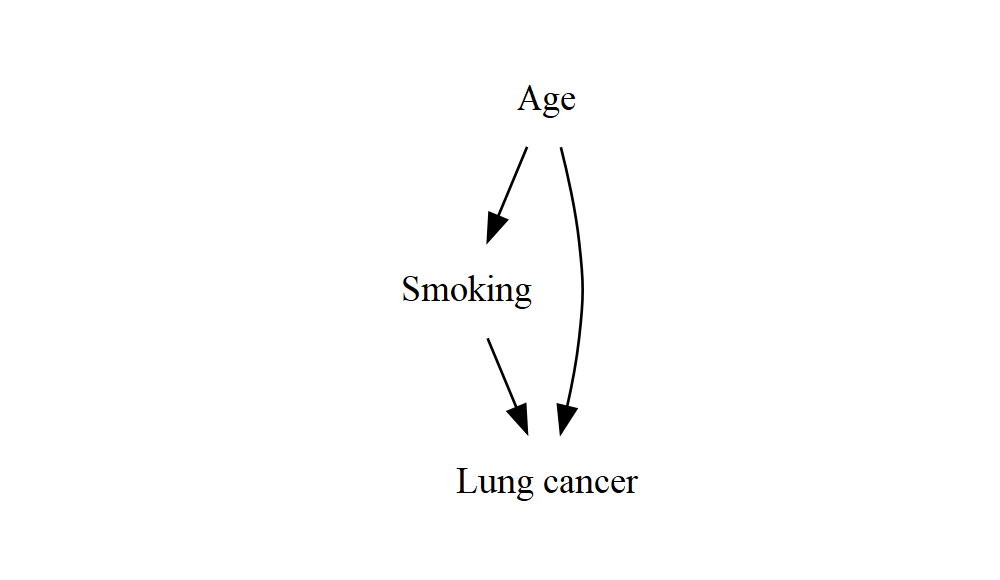
This is already not quite right, and as you add more variables it’ll quickly get even more out of hand. What I’d like to see is “Smoking” and “Lung cancer” next to each other, with an arrow going from left to right. They’re the stars of the show, and everything else should be around them in some way that makes it clear how it affects their relationship.

The layout algorithm of course has no idea what any of these things represent – it doesn’t know that “smoking” and “lung cancer” are the exposure and the outcome, and that they’re special somehow. At this point you’d be excused for thinking (as I initially did) that it must take a human to make these decisions, and thus we’re forced back to drag-and-drop tools. Luckily, it turns out that with just a couple of tricks we can get Graphviz/DiagrammeR to produce sensible results for even complex structures.

Vertically align nodes using rank

Fortunately, there’s a simple way to force two (or more) nodes to be vertically aligned (or in Graphviz terms, to have the same rank):

DiagrammeR::grViz("
digraph {
  graph []
  node [shape = plaintext]
    A [label = 'Smoking']
    Y [label = 'Lung cancer']
    C [label = 'Age']
  edge []
    A->Y
    C->A
    C->Y
  { rank = same; A; Y }
}
")

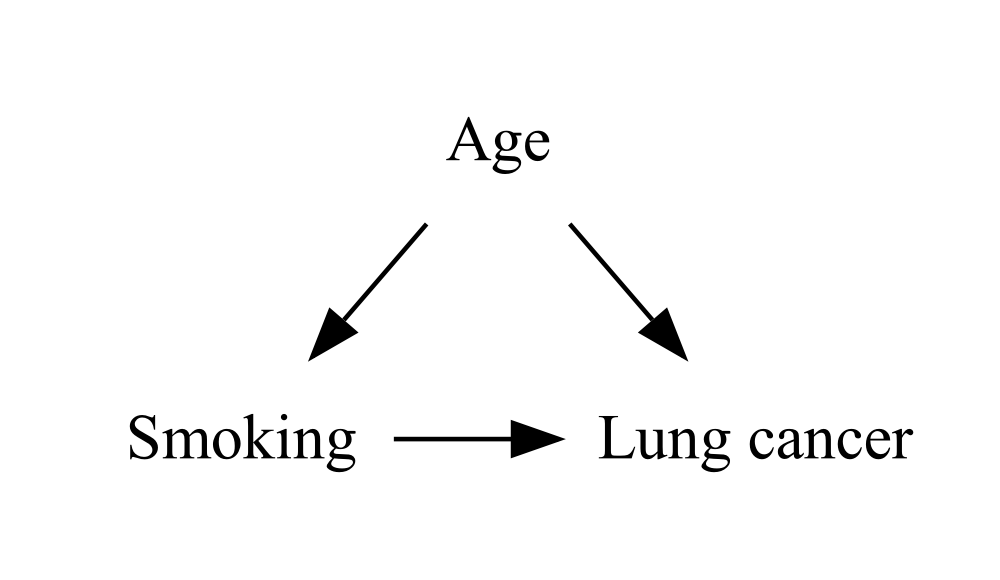
It turns out that this rank = same method goes a long, long way in keeping complicated causal structures looking reasonably sensible. Even with a very complex DAG, my experience so far is that as long as the exposure and outcome are aligned, the algorithm tends to find neat, sensible places to put everything else. If you do need to do more tweaking, you can add more of these statements, or use it to align more than two nodes:

DiagrammeR::grViz("
digraph {
  graph []
  node [shape = plaintext]
    A B C D Y
  edge []
    A->B->Y
    C->D->B
  { rank = same; A; B; Y }
  { rank = same; C; D }
}
")

You can also use min or max instead of same to force the nodes to be at the very top or the very bottom respectively (the layout goes from top to bottom, so the “minimum” is at the top):

DiagrammeR::grViz("
digraph {
  graph []
  node [shape = plaintext]
    A B C D Y
  edge []
    A->B->Y
    C->D->B
  { rank = min; A; B; Y }
  { rank = same; C; D }
}
")

Changing arrow lengths with minlen and ranksep

Something else might have bothered you about these examples by now: some of the arrows are very short. We can fix this by giving the edges a minlen (minimum length) attribute – if you wanted, you could set this individually for each edge by adding square brackets like we did with the nodes and labels, but I’ve done it for all the edges at once:

DiagrammeR::grViz("
digraph {
  graph []
  node [shape = plaintext]
    A [label = 'Smoking']
    Y [label = 'Lung cancer']
    C [label = 'Age']
  edge [minlen = 2]
    A->Y
    C->A
    C->Y
  { rank = same; A; Y }
}
")

This improved the horizontal arrow, but the diagonal arrows are now even longer! It seems that minlen controls the length both vertically and horizontally, but the units have a slightly different meaning for each one. Fortunately, we can control the vertical distance (the separation between each “rank”) independently by setting the ranksep attribute on the graph itself:

DiagrammeR::grViz("
digraph {
  graph [ranksep = 0.2]
  node [shape = plaintext]
    A [label = 'Smoking']
    Y [label = 'Lung cancer']
    C [label = 'Age']
  edge [minlen = 2]
    A->Y
    C->A
    C->Y
  { rank = same; A; Y }
}
")

In this case, it seems like a value of around 0.2 will make the vertical and horizontal arrows about the same length, no matter what minlen you choose. With a bigger and more complex graph, you might need to increase ranksep a bit.

Drawing boxes

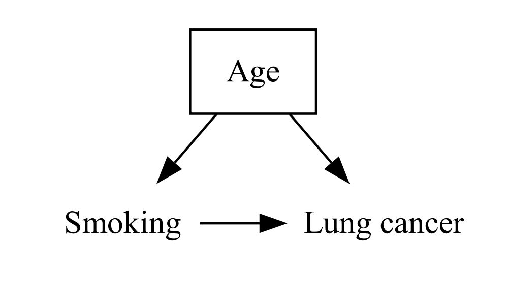
When we use causal diagrams in epidemiology, we usually draw a box around a variable to show that it’s been conditioned on or adjusted for, either by the study design or by the statistical analysis. Remember the shape parameter that we set to plaintext? We still want plaintext to be the default, but we can override it and set it to box for individual nodes:

DiagrammeR::grViz("
digraph {
  graph [ranksep = 0.2]
  node [shape = plaintext]
    A [label = 'Smoking']
    Y [label = 'Lung cancer']
    C [label = 'Age', shape = box]
  edge [minlen = 2]
    A->Y
    C->A
    C->Y
  { rank = same; A; Y }
}
")

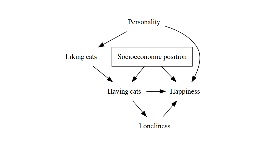
Summing up

Here’s a fuller example that uses all the tricks we’ve seen. I’ve added some extra blank lines to make the structure a bit clearer, and aligned all the labels – remember that line breaks and spacing are optional, but making good use of them to keep things tidy and readable will pay off whenever someone tries to understand your code (whether that’s just future you, or someone else).

DiagrammeR::grViz("
digraph {
  graph [ranksep = 0.2]

  node [shape = plaintext]
    A    [label = 'Having cats']
    Y    [label = 'Happiness']

    Lik  [label = 'Liking cats']
    Pers [label = 'Personality']
    Lon  [label = 'Loneliness']
    SEP  [label = 'Socioeconomic position', shape = box]

  edge [minlen = 2]
    A->Y

    Lik->A
    Pers->Lik
    Pers->Y

    A->Lon->Y

    SEP->A
    SEP->Y

  { rank = same; A; Y }
}
")

In summary:

• The structure of the graph is defined by the list of nodes and edges – everything else is more or less cosmetic.
• All the cosmetic stuff is done by setting attributes inside square brackets. You can set attributes for all nodes or edges at once by adding them in the brackets after node or edge, or for an individual node or edge by adding square brackets directly after it.
• Control how a node is displayed by giving it a label. If you don’t set a label, its name (A, Y, etc.) will show up instead.
• Draw a box around a node by adding shape = box to it.
• Vertically align nodes by adding, say, { rank = same; A; B; C } to vertically align nodes A, B and C.
• Change the length of the arrows by using a different value for minlen.
• If need be, set the length of an individual arrow by adding a minlen to a single edge definition, e.g. A->Y [minlen = 2].
• Change the vertical distance between rows by changing the value for ranksep – around 0.2 seems to make relatively small and uncomplicated graphs look balanced, but in a more complex diagram you might need to increase it.

And that’s about it. Enjoy drawing DAGs, and feel free to get in touch if you have any suggestions for improving or clarifying anything in this post.